If you are in VLSI industry, sometime or the other, you must have heard this term “Mont Carlo (MC)”. In this post let us understand the literal meaning of Monte Carlo simulation and its application in circuit design field. Going by the wiki definition of Monte Carlo “Monte Carlo methods are a broad class of computational algorithms that rely on repeated random sampling to obtain numerical results”. Simplifying the definition, Monte Carlo algorithms are used for introducing random variations within the given limits to explore the corner cases of any problem. The problems fed to Monte Carlo algorithms are spanned over a wide variety of applications including Risk Analysis, Finances, Statistics, Physics, and Electronic Designs.
This was pretty much the introduction of Monte Carlo. Now let’s get to the business and talk about WHY and HOW Monte Carlo algorithms are important in the VLSI design.
In VLSI circuit design during simulation, we run the design through various PVT (Process, Voltage and Temperature)corners with an aim that the circuit should be able to reliably operate at all the extreme conditions. These PVT variations can be generalized as,
- Temperature from as low as -40° to as high as 125°C,
- Voltage ±10% variation from its nominal value
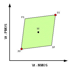
- Process – This is generally two letter convention where first letter is the behavior of NMOS and second letter is of PMOS. TT, SS, FF, SF and FS are the corners generally used. Letter T stands for Typical (Nominal Vt), F for Fast (Low Vt) and S for Slow (High Vt).
Running the design over different PVT corners cover the environmental variations (voltage and temperature) as well as manufacturing variations (process). A very common figure to illustrate the process corner is shown here,
Now the million dollar question is “Can we guarantee the functionality of silicon across all condition by simulating the design across PVT corners???”The answer comes out to be NO and guess what’s the reason??? It’s the manufacturing variations introduced during fabrication of the chip. But, didn’t we cover the manufacturing variations in the process corners (TT, SS, FF, FS and SF)? Yes, we did but that’s not enough. Let me explain !!!
Now just think about the scenario, we have a design which has 1000 NMOS and 1000 PMOS. Let’s say we are running this design at FS corner, considering all the 1000 NMOS are identically FAST and all the 1000 PMOS are identically SLOW. This is not true in real silicon where no two transistors are identical due to Systematic and Random variations. So even after running the design across process corners we are leaving behind the corner case where there is variations across different transistors in the same process corner. This is where Monte Carlo pitches in. It aids in introducing the randomness into the transistors by changing its Vt in different directions such that all the 1000 NMOS/PMOS are different at a time, depicting the real silicon behavior.
Industry-wide, the MC corner files itself are different than the usual process corner files for the reason that the variations at MC corners are different than the process corners hence one should avoid the mistake by running the MC at process corner, which will not be able to hit the worst case for above mentioned reasons.
The Monte Carlo simulations can be done in two ways for any given design, Global Monte and Local Monte. Again the corner files for these two will be different. Let’s understand what these are:
Global Monte: We can think of this Monte run as unconstrained in a way that the variations in this case can span over different process corners. Let’s understand this through a fig,
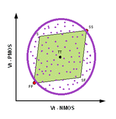
In the figure, each dot represents one Monte Carlo run and as we can see it will spread the variation by introducing a Vt change in its every single run. The span of the variations in this global Monte run is spread across the process corners as its name also suggests, Global MC.
Local MC: This Monte run is constrained to a particular process corner. In general, first step is to run the design at various PVT coroners to find the worst one. Then second step is to run the Monte on this particular corner to see the functionality on worst of worst corner. Let us say the worst corner in the first step was found to be SS then the Monte variations will look something like this,
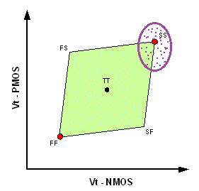
This is Local Monte as the scope of variations is limited to a particular corner.
Both the methods have their own set of applications and used across industry to emulate the silicon behavior during simulation and have a working silicon in one go. Undoubtedly, The Mysterious Monte Carlo has many flavors or to say applications and I hope now you can appreciate the use of it to just another application, VLSI Circuit Design !!!